Fancy Headers in Automated Reports

Using RMarkdown with knitr is a great way of automating reports under R and I’ve used this approach extensively in shiny apps. For one particular project we’re storing raw data in a SQL database and processing on the fly under shiny. Results are displayed using heatmaps and graphs. We’re now considering pushing data reports to a filestore that connects to another corporate database via a visualizer. Not wanting to generate extra work, this is a great opportunity to put rmarkdown and knitr to work. I’ve added some code to the upload so that each time data are uploaded to the database some rudimentary calculations are performed and a pdf report is automatically generated. Unlike many of the other reports I’ve put together in the past, this one requires the title to be placed in a header along with a link to the app for further processing.
All this can be achieved with a little programming in R and latex as shown below…

Here is a snippet from the app.R code. In this case ASSAY_TITLE refers to the name of the assay. Data have already been processed and are stored in a reactive variable (df.raw), comprising of Sample, Concentration and several columns of processed data.

  ## Generate reports
  observeEvent(input$butReport, {
    req(df.raw())
    for (sample in unique(df.raw()$Sample)) {  ## Create one report for each sample
      output_file <- paste(sample, Sys.Date(), 'ASSAY_TITLE', "FA.pdf", sep='_')
      file_with_path <- paste(tempdir(), output_file, sep = '/')
      rmarkdown::render(input = "./upload_report.Rmd",
              output_format = "pdf_document",
              output_file = output_file,
              output_dir = tempdir(),
              params=list(sample=sample,  ## Send parameters to markdown yaml
                          date=Sys.Date()))
      df$report[df$report$Sample == sample, 'Uploaded'] <- TRUE
      ## send report to filestore
      inq_metadata <- '{"file_content": "Report", "description": "ASSAY_TITLE Report file"}'
      uploadFile(parent_id, file_with_path, metadata = inq_metadata)
    }
  })

Here’s the entire rmarkdown file. The yaml at the top contains a params line to pass paraneters from the ramarkdown::render command. Two variables are set in yaml - the title and author - these contain data which will be used for two lines in the header. The author is used to store the subtitle data and consists of an r paste0 command concatenating teh sample name and date (passed as variables). A couple of latex packages are included: graphicx to include a graphic and fancyhdr to manage creating a header. The statement that reads \AtBeginDocument{\let\maketitle\relax} allows us to define the title in yaml but does not automatically print it to the document title page. The latex code defines a header/footer for the plain page style. The footer contains the page number, centered and the header contains the title and author variables, left justified, with the title on top. In addition to the title information in the header, a graphic is included, right justified. The graphic is embedded in an \href command and links to the app. This allows the user to view the report which contains limited information and click to the app for further detail. Once this is all in place, all that is needed is to issue a \newpage followed by \pagestyle{plain} at the start of each page.

---
params: 
  sample: ""
  date: ""
title: "FATTY ACID ANALYSIS"
author: "`r paste0('Sample: ', params$sample, ' --- Uploaded: ', params$date)`"
header-includes:
  \usepackage{graphicx}
  \usepackage{fancyhdr}
  \AtBeginDocument{\let\maketitle\relax}
output: pdf_document
---

\makeatletter
\fancypagestyle{plain}{
  \fancyhf{}
  \fancyfoot[C]{\thepage}
  \fancyhead[L]{\Large \textbf{\@title} \\ \large \@author}
  \fancyhead[R]{\href{http://link_to_shiny_app/}{\includegraphics{link_button.png}}}
}

\pagestyle{plain}
\vspace*{1\baselineskip}

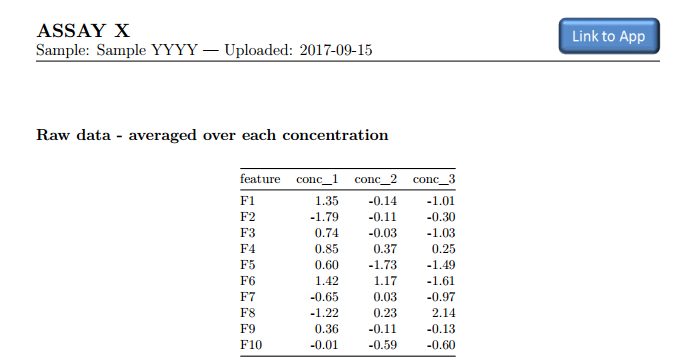
## Raw data - averaged over each concentration
```{r, results='asis'}

df.tab1 <- df.raw() %>%
  filter(Sample == sample) %>%
  select(-Sample) %>%
  gather(FA, Value, -Conc) %>%
  group_by(FA, Conc) %>%
  summarise(av_Conc = round(mean(Value), 3)) %>%
  spread(Conc, av_Conc)
names(df.tab1)[-1] <- paste(names(df.tab1)[-1], 'µM')
kable(df.tab1)

```
\newpage
\pagestyle{plain}

## Normalized data - averaged over each concentration
```{r results='asis'}

features <- names(df.raw())[-c(1:2)]
df.tab2 <- df.raw() %>%
  filter(Sample == sample) %>%
  select(-Sample) %>%
  mutate(total = rowSums(.[-1], na.rm = TRUE)) %>%
  mutate_at(features, funs(100*./total)) %>%
  select(-total) %>%
  gather(FA, Value, -Conc) %>%
  group_by(FA, Conc) %>%
  summarise(av_Conc = round(mean(Value), 3)) %>%
  spread(Conc, av_Conc)
names(df.tab2)[-1] <- paste(names(df.tab2)[-1], 'µM')
kable(df.tab2)

```